Restoring Identity: How Manifold Constraints Tame the Hyper-Connection Chaos
I’ve been reading through the new paper “mHC: Manifold-Constrained Hyper-Connections” (arXiv:2512.24880), and honestly, it feels like finding a missing puzzle piece for modern Deep Learning architectures.
We’ve all gotten used to ResNets and Transformers dominating the landscape. The secret sauce? Residual Connections. That simple x + F(x) is the reason we can train 100-layer networks without gradients vanishing into oblivion.
But recently, people started asking: Why just a simple addition? Why not make the residual stream wider, smarter, and more complex? Enter Hyper-Connections (HC). They sounded great on paper—expanding the residual highway to carry more info. But there was a catch. As you go deeper, things explode. The model becomes unstable.
This paper proposes a fix that is so mathematically elegant it hurts: Manifold Constraints.
Let’s break it down.
1. The Overview: The “Identity Crisis” of Hyper-Connections
To understand mHC, we first need to understand the problem with standard Hyper-Connections.
The Original Superpower: Identity Mapping
In a classic ResNet or Transformer, the residual connection is an Identity Mapping. It preserves the signal. If you have a signal $x$, and you add nothing to it, it stays $x$. This is crucial because it allows gradients to flow straight through the network, like a superhighway with no toll booths.
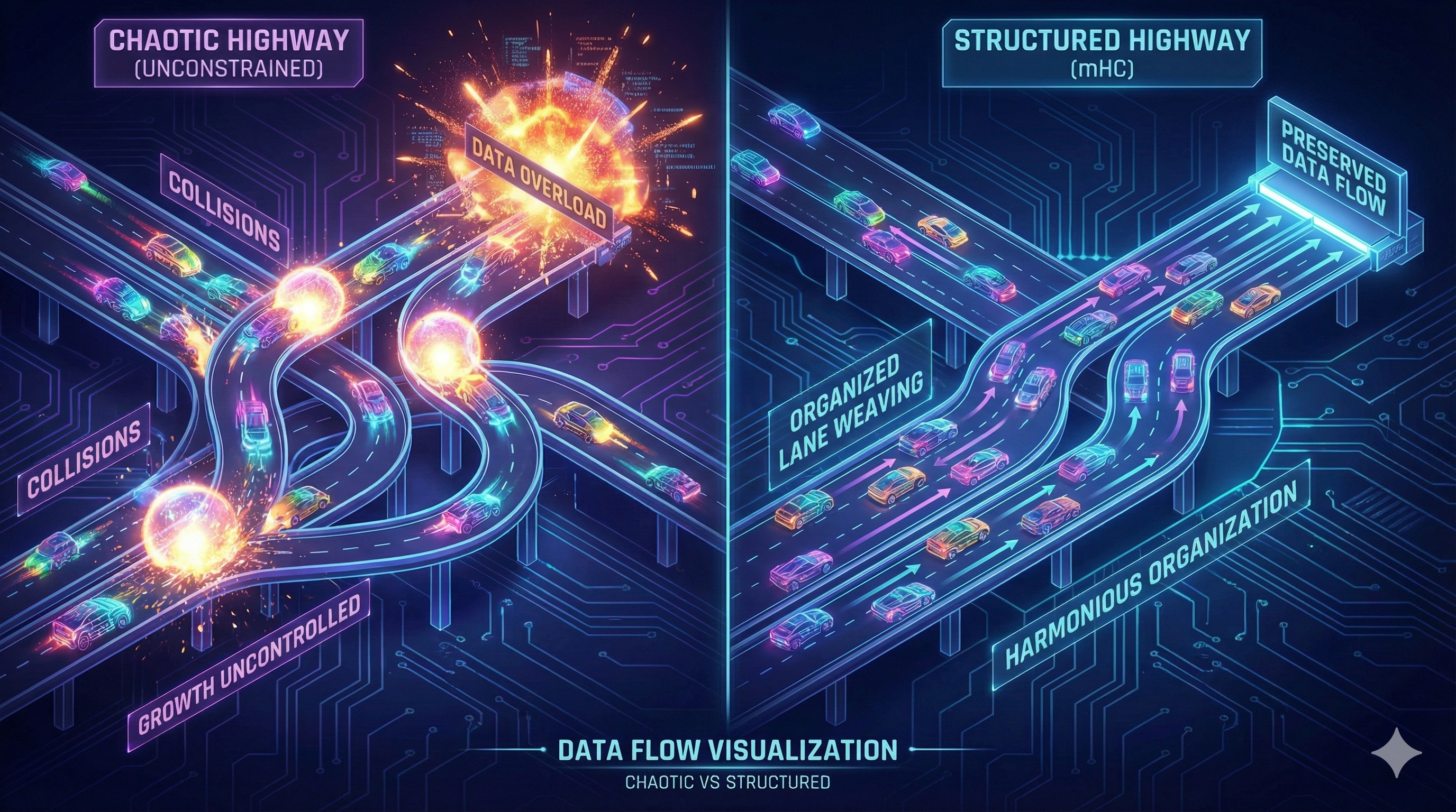
Hyper-Connections (HC) tried to upgrade this highway. Instead of a single lane (dimension $C$), they expanded it to multiple lanes (dimension $n \times C$) and added “mixers” ($\mathcal{H}^{res}$) to shuffle traffic between lanes.
The Problem: The runaway Train
The issue is that these “mixers” were unconstrained. Imagine a highway where every time you switch lanes, your car gets slightly faster. By the time you reach layer 50, you aren’t driving; you’re breaking the sound barrier.
Mathematically, multiplying random matrices layer after layer leads to signal explosion (values get too big) or signal vanishing (values get too small). The “Identity” property—the safety net—is lost. Your model becomes unstable, and training collapses at scale.
The Solution: mHC
The authors introduce Manifold-Constrained Hyper-Connections (mHC). They said: “Okay, let’s keep the multi-lane highway, but let’s strictly enforce the rules of physics.”
They force the mixing matrices to live on a specific Manifold—specifically, the manifold of Doubly Stochastic Matrices.
What does that mean? It means the total amount of “signal energy” entering the mixer must equal the amount leaving it. No free energy. No explosions. Just pure, stable mixing.
2. A Deep Dive into the Maths (The Evolution of Identity)
To truly appreciate mHC, we need to trace the evolution of the “residual connection” and see exactly where the math breaks—and how mHC fixes it.
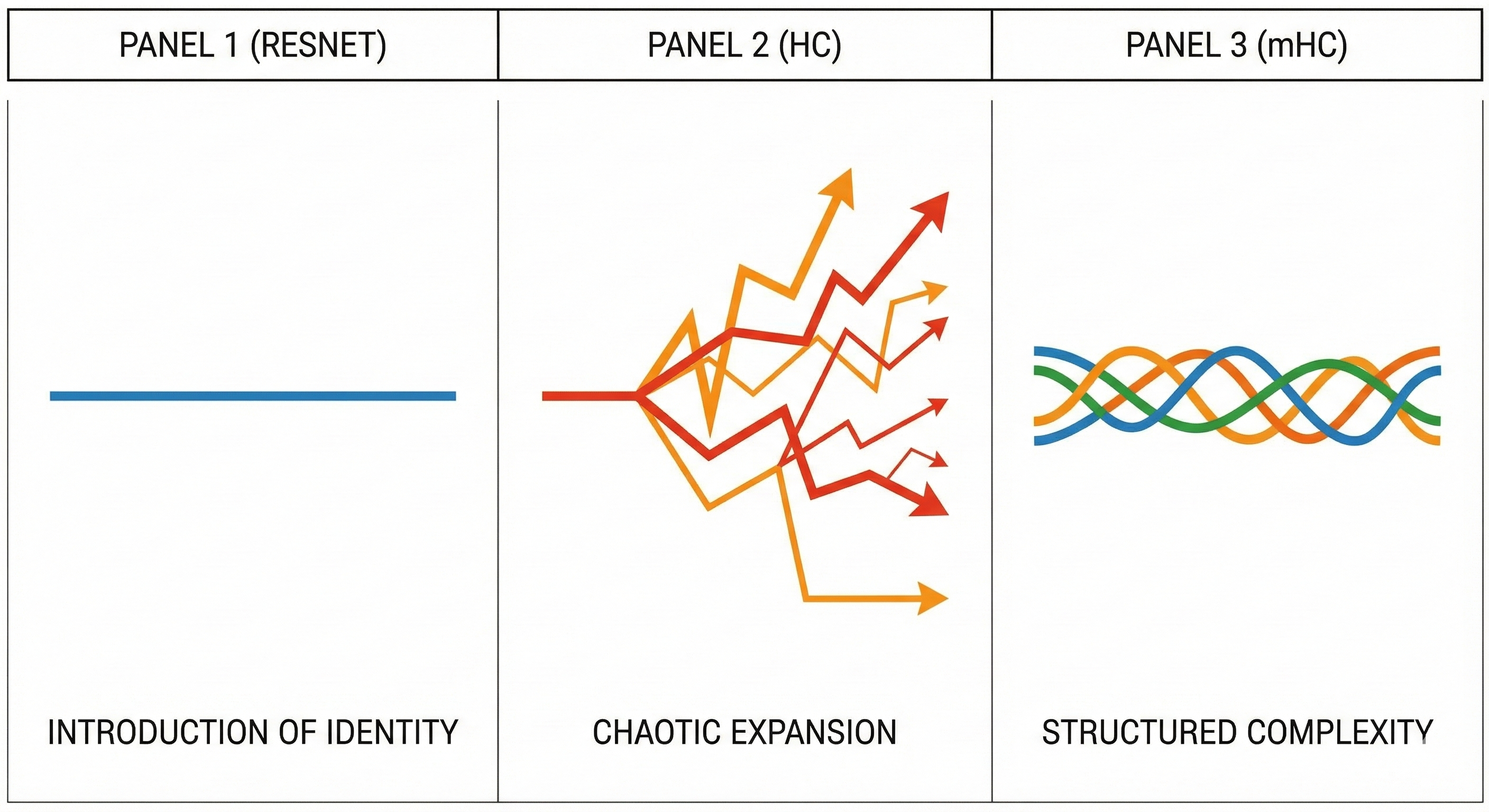
Let’s look at three evolutionary stages.
Stage 1: The Classic Residual Connection (Addition)
In a standard ResNet or Transformer, the equation for a layer is simple addition:
\[\mathbf{x}_{l+1} = \mathbf{x}_l + \mathcal{F}(\mathbf{x}_l)\]Here, $\mathcal{F}$ is your attention or feed-forward block. The critical part is the $\mathbf{x}_l$ term. It has a coefficient of 1. If we stack $L$ layers, the signal can propagate all the way from the start to the end: \(\mathbf{x}_L = \mathbf{x}_0 + \sum_{i=0}^{L-1} \mathcal{F}(\mathbf{x}_i)\)
The Intuition: This is like a conveyor belt moving at a constant speed. You can drop packages ($\mathcal{F}$) onto it, but the belt itself ($\mathbf{x}_l$) keeps moving steadily. It doesn’t speed up or slow down. Stability is guaranteed because $1 \times 1 \times 1 \dots = 1$.
Stage 2: Hyper-Connections (Matrix Multiplication)
Hyper-Connections (HC) wanted to make the conveyor belt smarter. Instead of just carrying the signal forward, they wanted to mix information between different “lanes” (expanded dimensions). So, they replaced the simple addition with a matrix multiplication:
\[\mathbf{x}_{l+1} = \mathcal{H}^{res}_l \mathbf{x}_l + \mathcal{F}(\mathbf{x}_l)\]Here, $\mathcal{H}^{res}_l$ is a learnable $n \times n$ matrix. Now, look what happens when we stack layers. Instead of a sum, we get a product:
\[\mathbf{x}_L = \left( \prod_{i=0}^{L-1} \mathcal{H}^{res}_i \right) \mathbf{x}_0 + \dots\]The Intuition (and the Problem): This is no longer a steady conveyor belt. It’s a series of gearboxes.
- If $\mathcal{H}^{res}$ effectively multiplies the signal by $1.1$, after 100 layers, your signal is $1.1^{100} \approx 13,000$ times stronger. (Explosion)
- If it multiplies by $0.9$, your signal becomes $0.9^{100} \approx 0.00002$. (Vanishing)
This is why HC models are unstable. The “Identity” is lost because the product of random matrices rarely stays close to 1.
Stage 3: Manifold-Constrained Hyper-Connections (mHC)
This is the paper’s “Galaxy Brain” moment. They realized we can keep the complex mixing of HC, but force it to behave like the steady conveyor belt of Stage 1.
They constrain $\mathcal{H}^{res}$ to be a Doubly Stochastic Matrix.
Mathematically, this means:
- All entries are non-negative: $\mathcal{H}_{ij} \ge 0$
- Rows sum to 1: $\sum_j \mathcal{H}_{ij} = 1$
- Columns sum to 1: $\sum_i \mathcal{H}_{ij} = 1$
Why does this specific constraint matter? Because of the Spectral Norm. For any doubly stochastic matrix $M$, its largest eigenvalue is exactly 1. \(\|\mathcal{H}^{res}\|_2 \le 1\)
And crucially, the product of two doubly stochastic matrices is also doubly stochastic. \(\text{Product} = \prod \mathcal{H}^{res}_i \implies \text{Still Doubly Stochastic}\)
The Intuition: Think of the signal as water flowing through pipes.
- HC was leaky pipes where water could randomly be added or lost at every junction.
- mHC is a closed system. The water can split into different pipes, swirl around, and mix (that’s the “Hyper” connectivity), but not a single drop is created or destroyed.
By projecting the weights onto this “Manifold” (the Birkhoff Polytope), they mathematically guarantee that the signal cannot explode, no matter how deep the network gets. It restores the “Identity Mapping” property while still allowing for complex feature mixing.
How They Actually Implement It (Sinkhorn-Knopp)
You might wonder, “How do you train a neural net to output Doubly Stochastic matrices?” You don’t. You let it output whatever it wants, and then you “fix” it on the fly using the Sinkhorn-Knopp algorithm.
It’s an iterative normalization:
- Take raw weights $W$.
- Exponentiate to make them positive: $e^W$.
- Alternately normalize rows and columns to sum to 1.
After about 20 iterations, it converges to the perfect manifold. This fits right into the forward pass, making the stability a structural guarantee rather than a lucky training outcome.
3. The “Kernel-Hacking” You Didn’t See Coming
The authors didn’t just stop at the math. They realized that implementing this on actual GPUs is a nightmare because of memory bandwidth. So they went full “Kernel Hacker” mode (Section 4.3).
The Problem: RMSNorm is a Diva
Normally, you do MatMul -> RMSNorm. But RMSNorm is slow and memory-hungry when dealing with these expanded hyper-states ($n \times C$). It imposes significant latency.
The Fix: Fusion & Reordering
They realized they could mathematically reorder the operations. Instead of normalizing after the huge matrix multiplication, they fused it into the kernel itself. They used TileLang (a custom kernel language) to write fused GPU kernels that:
- Fuse Projections + Bias + Norm into a single operation.
- Fuse the Sinkhorn-Knopp iterations into a single kernel launch.
- Fuse the backward pass so it doesn’t need to reload data.
This is the equivalent of turning a 5-step recipe into a single button press.
The “Free Lunch” Memory Hack
Because Hyper-Connections use $N$ streams, they chew up $N$ times more memory, right? Wrong. They implemented On-the-Fly Recomputing. During backpropagation, instead of storing all the massive intermediate states in VRAM (which would crash your H100s), they efficiently re-calculate the mHC kernels on demand. Because they optimized the kernels so heavily, re-computing them is actually cheaper than the memory cost of storing them.
The Math Behind the Speed
The authors didn’t just wave their hands; they calculated exactly how much memory bandwidth they saved by fusing operations.
Let $C$ be the channel dimension and $n$ be the number of streams (usually 4).
Before Optimization (Standard HC): To apply the mixing coefficients, you need to read the inputs, the pre-mixing weights, and the post-mixing weights.
- Reads: $(3n + 1)C$ elements.
- Writes: $3nC$ elements (intermediate results).
After Optimization (Fused mHC): By fusing everything into one kernel and merging operations, they cut this down drastically.
- Reads: $(n + 1)C$ elements.
- Writes: $nC$ elements.
Let’s plug in $n=4$:
- Reads: Reduced from $13C \to 5C$ (2.6x fewer reads)
- Writes: Reduced from $12C \to 4C$ (3x fewer writes)
This is why the training overhead is only 6.7%. They are doing more math (complex manifold projections) but less memory movement. In the GPU world, math is free, but memory movement is expensive. They traded the free resource for the expensive one.
The result? They scaled this to 27 Billion Parameters with only a 6.7% training overhead. That is insane efficiency for such a complex toplogy.
Why This Matters?
- Stability: They showed that mHC reduces the gradient explosion by 3 orders of magnitude compared to standard HC.
- Performance: It outperforms baselines on tough reasoning tasks (MMLU, GSM8K).
- Scalability: It allows us to build wider, more interconnected models without them falling apart.
It basically lets us have our cake (complex hyper-connections) and eat it too (training stability).
Understanding the Future
Papers like this remind me that we are still figuring out the fundamental “physics” of neural networks. We started with simple connections, broke them to make them “Hyper”, and are now using geometry (manifolds) to fix them.
It makes you wonder: what other geometric constraints are we missing that could unlock the next generation of 100 Trillion parameter models?
Images were generated using Google’s Nano Banana Pro.