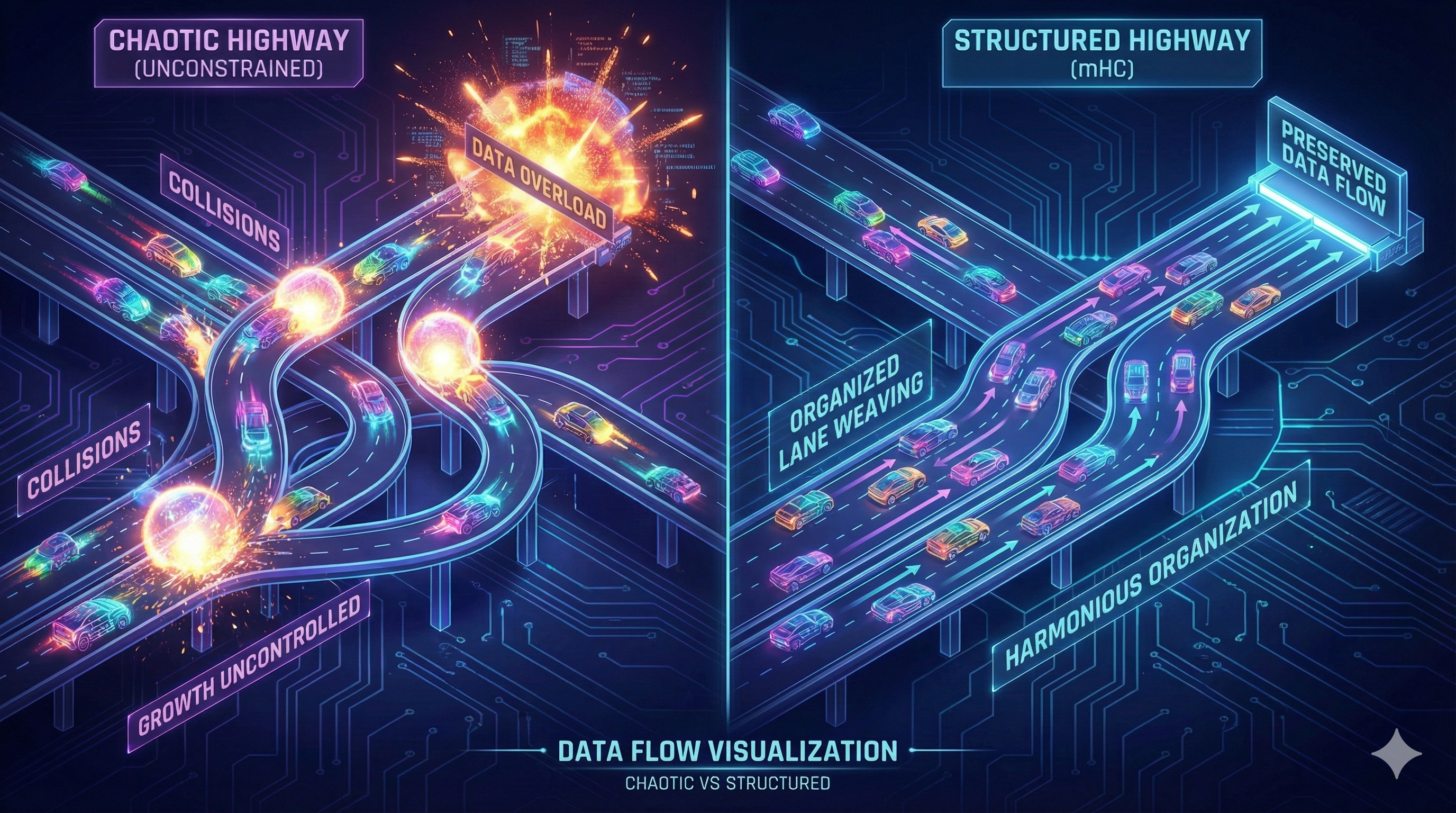
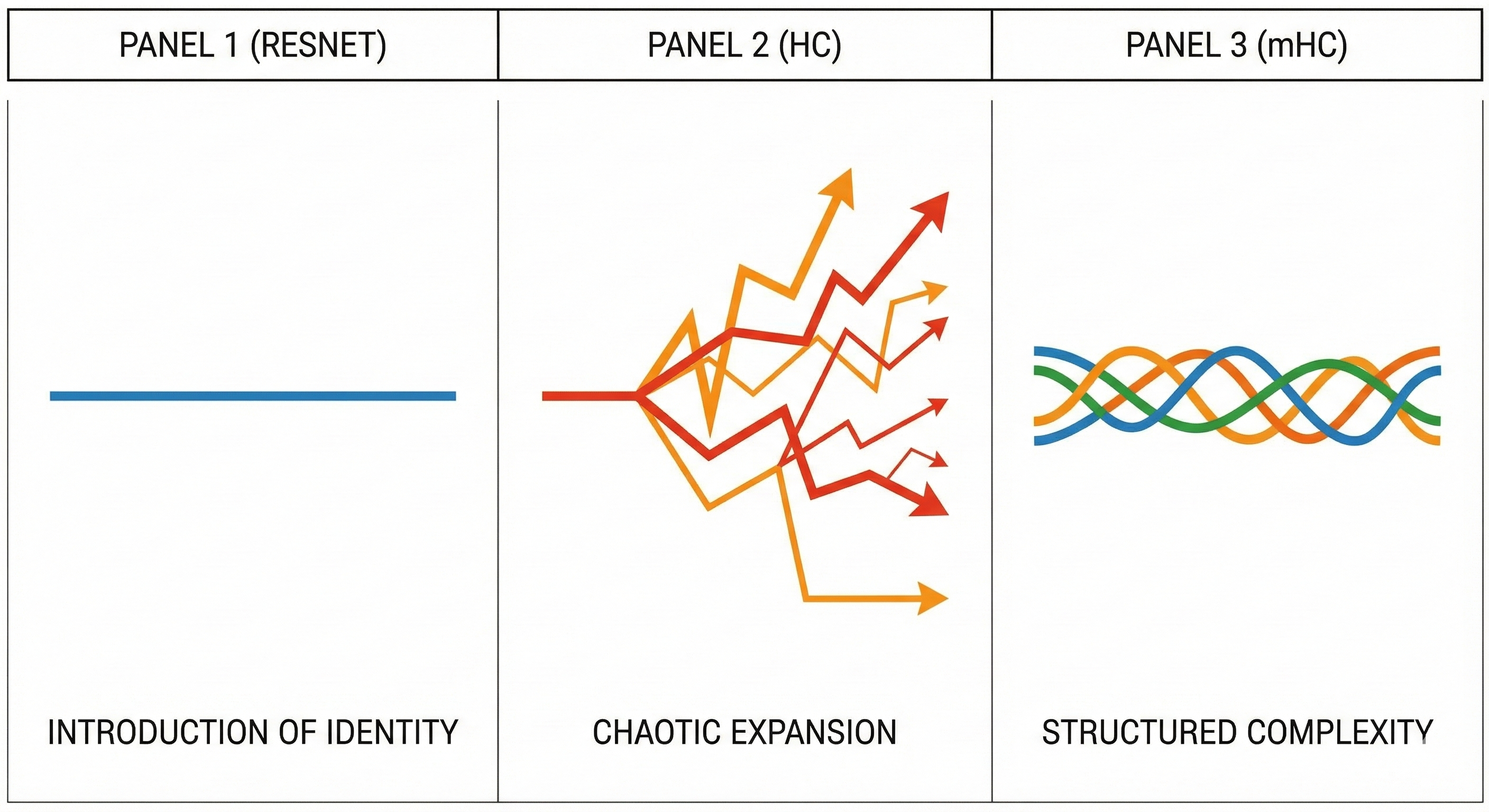
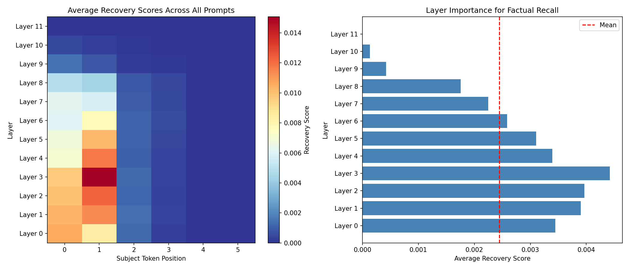
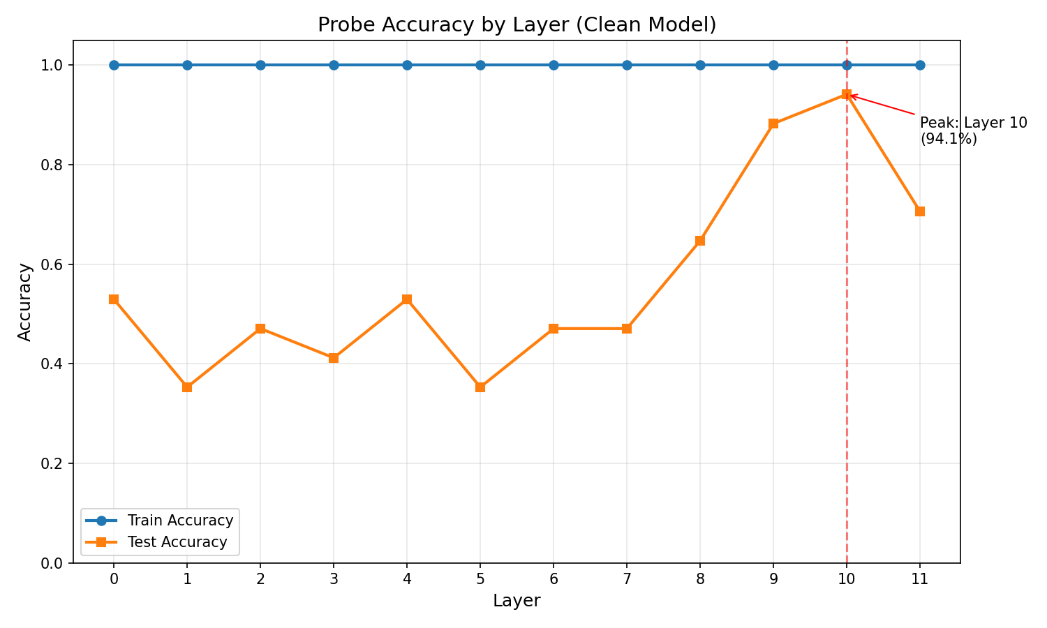
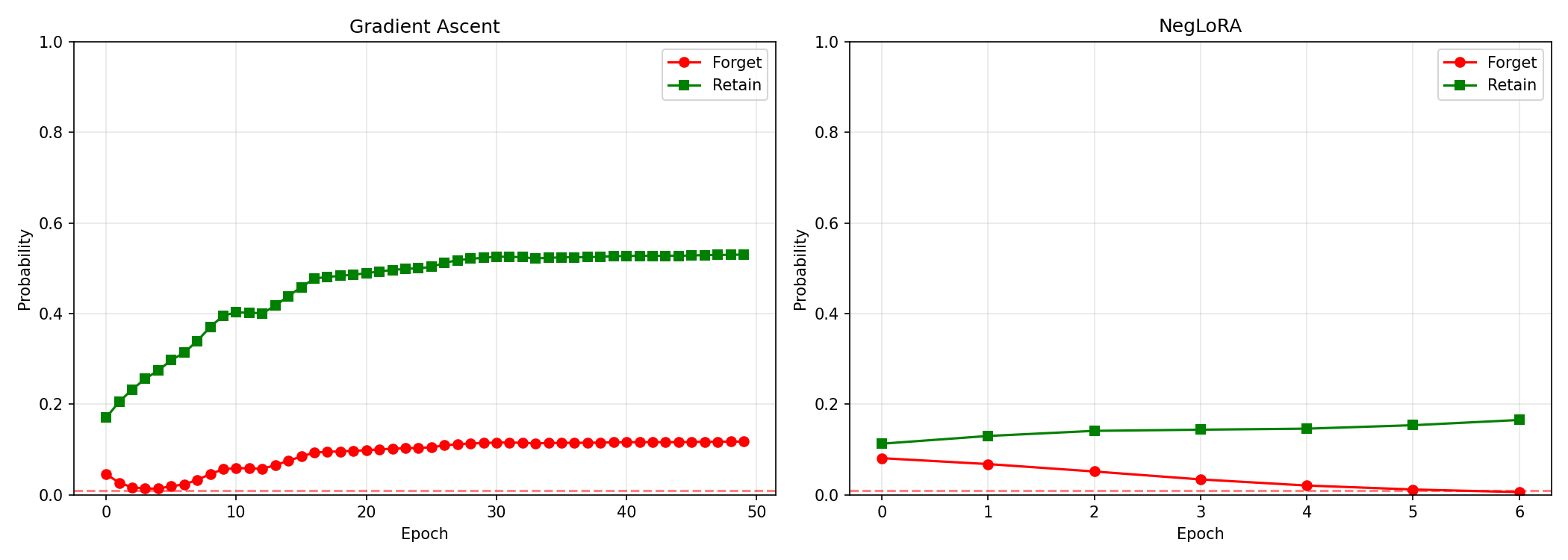
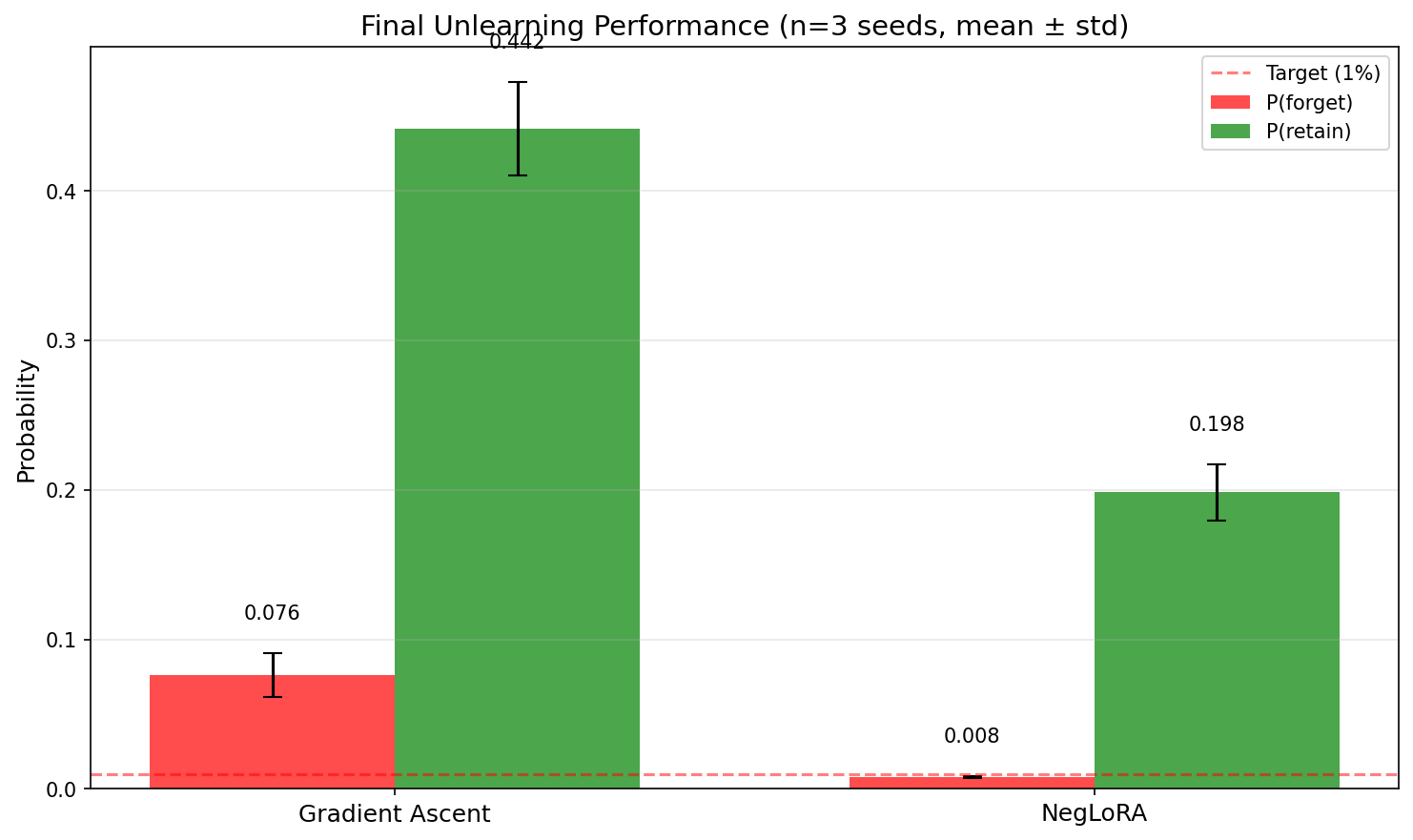
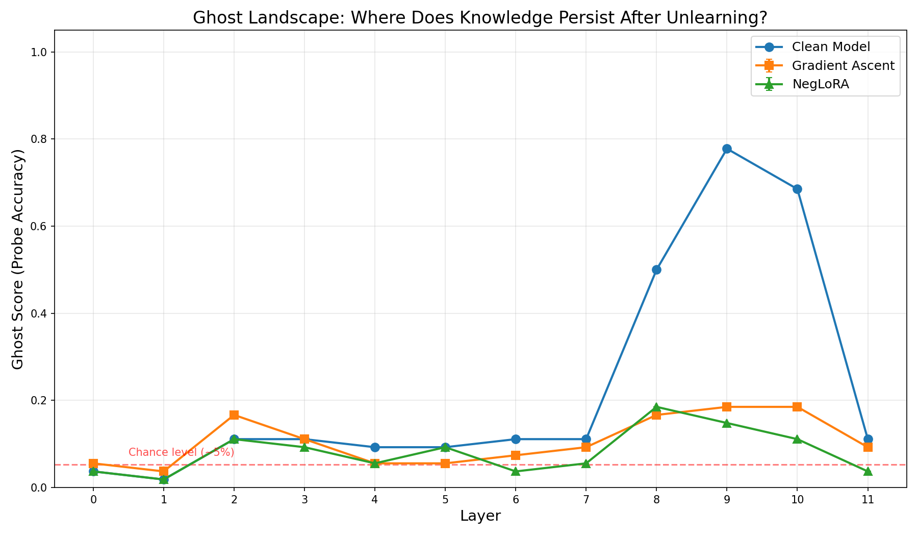
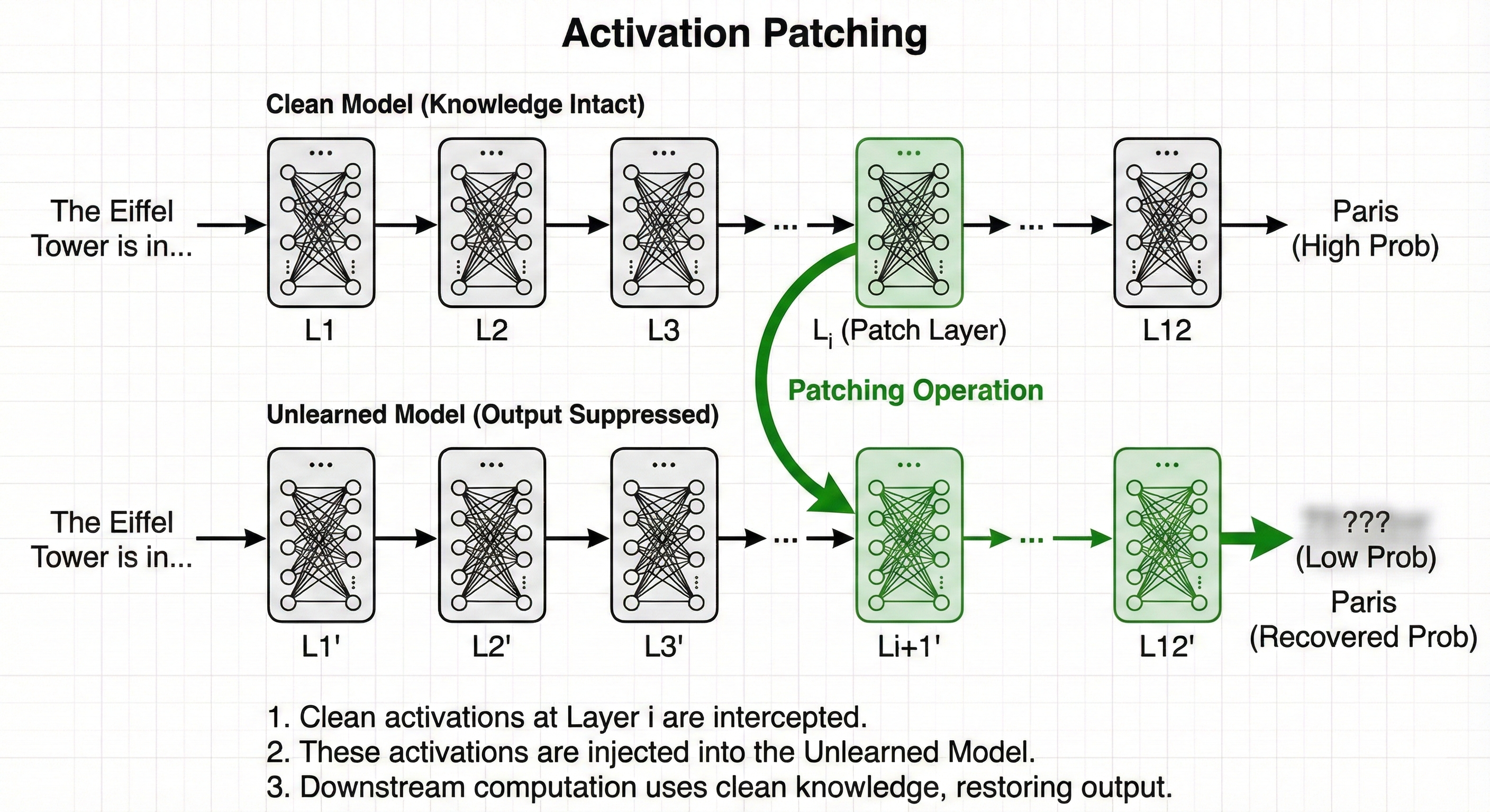
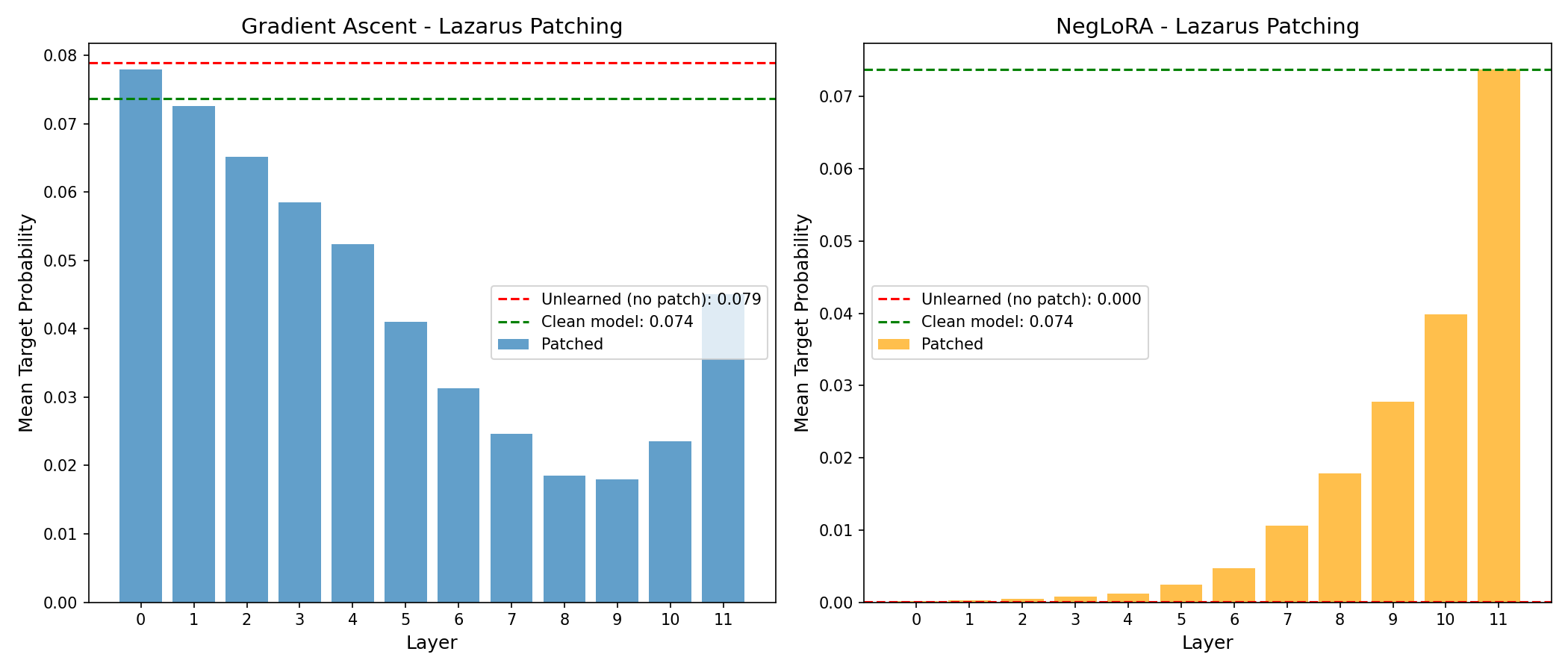
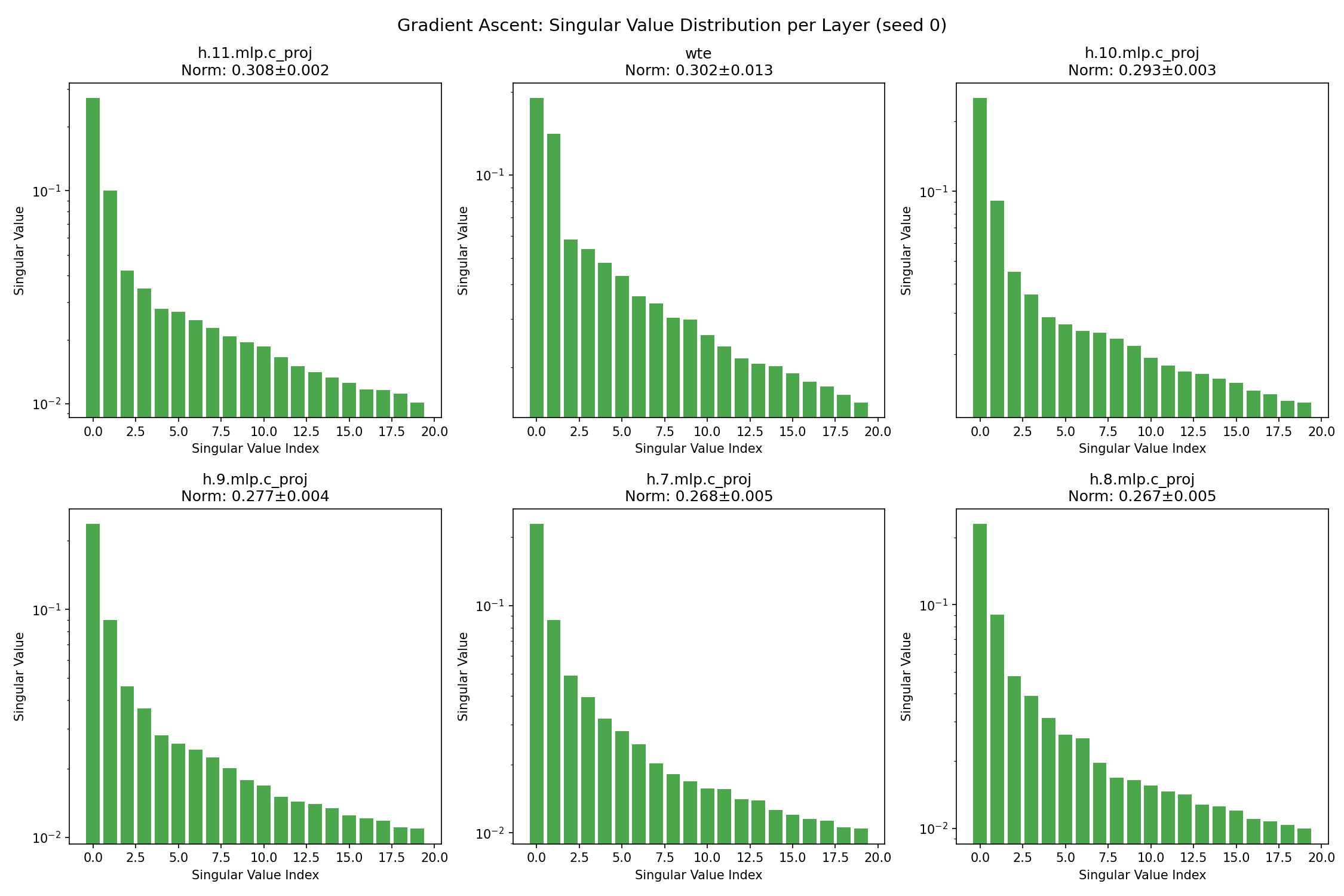
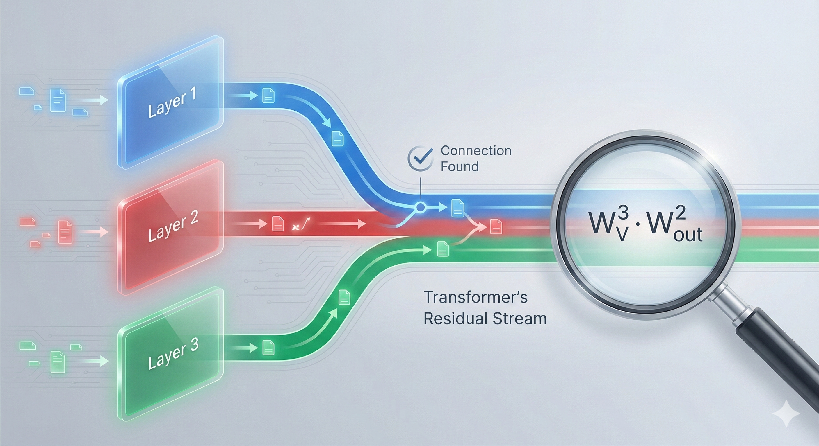
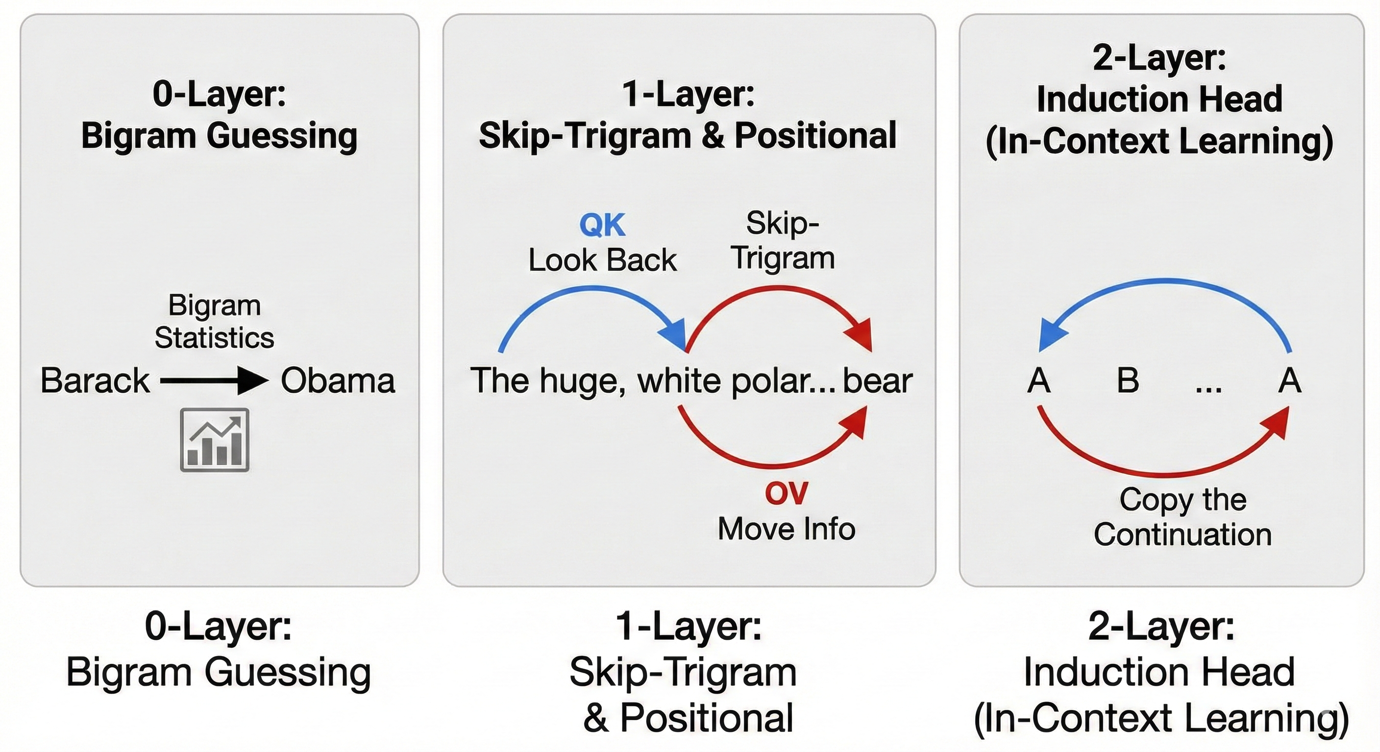
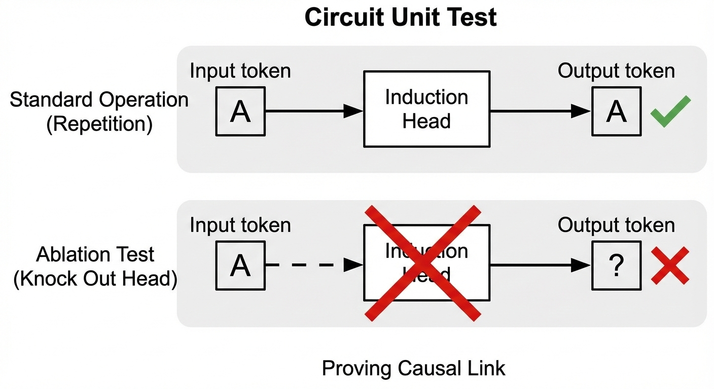
We’ve all gotten used to ResNets and Transformers dominating the landscape. The secret sauce? Residual Connections. That simple x + F(x) is the reason we can train 100-layer networks without gradients vanishing into oblivion.

But recently, people started asking: Why just a simple addition? Why not make the residual stream wider, smarter, and more complex? Enter Hyper-Connections (HC). They sounded great on paper—expanding the residual highway to carry more info. But there was a catch. As you go deeper, things explode. The model becomes unstable.

This paper proposes a fix that is so mathematically elegant it hurts: Manifold Constraints.

Let’s break it down.

1. The Overview: The “Identity Crisis” of Hyper-Connections

To understand mHC, we first need to understand the problem with standard Hyper-Connections.

The Original Superpower: Identity Mapping

In a classic ResNet or Transformer, the residual connection is an Identity Mapping. It preserves the signal. If you have a signal $x$, and you add nothing to it, it stays $x$. This is crucial because it allows gradients to flow straight through the network, like a superhighway with no toll booths.

Hyper-Connections (HC) tried to upgrade this highway. Instead of a single lane (dimension $C$), they expanded it to multiple lanes (dimension $n \times C$) and added “mixers” ($\mathcal{H}^{res}$) to shuffle traffic between lanes.

The Problem: The runaway Train

The issue is that these “mixers” were unconstrained. Imagine a highway where every time you switch lanes, your car gets slightly faster. By the time you reach layer 50, you aren’t driving; you’re breaking the sound barrier.

Mathematically, multiplying random matrices layer after layer leads to signal explosion (values get too big) or signal vanishing (values get too small). The “Identity” property—the safety net—is lost. Your model becomes unstable, and training collapses at scale.

The Solution: mHC

The authors introduce Manifold-Constrained Hyper-Connections (mHC). They said: “Okay, let’s keep the multi-lane highway, but let’s strictly enforce the rules of physics.”

They force the mixing matrices to live on a specific Manifold—specifically, the manifold of Doubly Stochastic Matrices.

What does that mean? It means the total amount of “signal energy” entering the mixer must equal the amount leaving it. No free energy. No explosions. Just pure, stable mixing.

2. A Deep Dive into the Maths (The Evolution of Identity)

To truly appreciate mHC, we need to trace the evolution of the “residual connection” and see exactly where the math breaks—and how mHC fixes it.

Let’s look at three evolutionary stages.

Stage 1: The Classic Residual Connection (Addition)

In a standard ResNet or Transformer, the equation for a layer is simple addition:

Here, $\mathcal{F}$ is your attention or feed-forward block. The critical part is the $\mathbf{x}_l$ term. It has a coefficient of 1. If we stack $L$ layers, the signal can propagate all the way from the start to the end: \(\mathbf{x}_L = \mathbf{x}_0 + \sum_{i=0}^{L-1} \mathcal{F}(\mathbf{x}_i)\)

The Intuition: This is like a conveyor belt moving at a constant speed. You can drop packages ($\mathcal{F}$) onto it, but the belt itself ($\mathbf{x}_l$) keeps moving steadily. It doesn’t speed up or slow down. Stability is guaranteed because $1 \times 1 \times 1 \dots = 1$.

Stage 2: Hyper-Connections (Matrix Multiplication)

Hyper-Connections (HC) wanted to make the conveyor belt smarter. Instead of just carrying the signal forward, they wanted to mix information between different “lanes” (expanded dimensions). So, they replaced the simple addition with a matrix multiplication:

Here, $\mathcal{H}^{res}_l$ is a learnable $n \times n$ matrix. Now, look what happens when we stack layers. Instead of a sum, we get a product:

The Intuition (and the Problem): This is no longer a steady conveyor belt. It’s a series of gearboxes.

• If $\mathcal{H}^{res}$ effectively multiplies the signal by $1.1$, after 100 layers, your signal is $1.1^{100} \approx 13,000$ times stronger. (Explosion)
• If it multiplies by $0.9$, your signal becomes $0.9^{100} \approx 0.00002$. (Vanishing)

This is why HC models are unstable. The “Identity” is lost because the product of random matrices rarely stays close to 1.

Stage 3: Manifold-Constrained Hyper-Connections (mHC)

This is the paper’s “Galaxy Brain” moment. They realized we can keep the complex mixing of HC, but force it to behave like the steady conveyor belt of Stage 1.

They constrain $\mathcal{H}^{res}$ to be a Doubly Stochastic Matrix.

Mathematically, this means:

1. All entries are non-negative: $\mathcal{H}_{ij} \ge 0$
2. Rows sum to 1: $\sum_j \mathcal{H}_{ij} = 1$
3. Columns sum to 1: $\sum_i \mathcal{H}_{ij} = 1$

Why does this specific constraint matter? Because of the Spectral Norm. For any doubly stochastic matrix $M$, its largest eigenvalue is exactly 1. \(\|\mathcal{H}^{res}\|_2 \le 1\)

And crucially, the product of two doubly stochastic matrices is also doubly stochastic. \(\text{Product} = \prod \mathcal{H}^{res}_i \implies \text{Still Doubly Stochastic}\)

The Intuition: Think of the signal as water flowing through pipes.

• HC was leaky pipes where water could randomly be added or lost at every junction.
• mHC is a closed system. The water can split into different pipes, swirl around, and mix (that’s the “Hyper” connectivity), but not a single drop is created or destroyed.

By projecting the weights onto this “Manifold” (the Birkhoff Polytope), they mathematically guarantee that the signal cannot explode, no matter how deep the network gets. It restores the “Identity Mapping” property while still allowing for complex feature mixing.

How They Actually Implement It (Sinkhorn-Knopp)

You might wonder, “How do you train a neural net to output Doubly Stochastic matrices?” You don’t. You let it output whatever it wants, and then you “fix” it on the fly using the Sinkhorn-Knopp algorithm.

It’s an iterative normalization:

1. Take raw weights $W$.
2. Exponentiate to make them positive: $e^W$.
3. Alternately normalize rows and columns to sum to 1.

After about 20 iterations, it converges to the perfect manifold. This fits right into the forward pass, making the stability a structural guarantee rather than a lucky training outcome.

3. The “Kernel-Hacking” You Didn’t See Coming

The authors didn’t just stop at the math. They realized that implementing this on actual GPUs is a nightmare because of memory bandwidth. So they went full “Kernel Hacker” mode (Section 4.3).

The Problem: RMSNorm is a Diva

Normally, you do MatMul -> RMSNorm. But RMSNorm is slow and memory-hungry when dealing with these expanded hyper-states ($n \times C$). It imposes significant latency.

The Fix: Fusion & Reordering

They realized they could mathematically reorder the operations. Instead of normalizing after the huge matrix multiplication, they fused it into the kernel itself. They used TileLang (a custom kernel language) to write fused GPU kernels that:

1. Fuse Projections + Bias + Norm into a single operation.
2. Fuse the Sinkhorn-Knopp iterations into a single kernel launch.
3. Fuse the backward pass so it doesn’t need to reload data.

This is the equivalent of turning a 5-step recipe into a single button press.

The “Free Lunch” Memory Hack

Because Hyper-Connections use $N$ streams, they chew up $N$ times more memory, right? Wrong. They implemented On-the-Fly Recomputing. During backpropagation, instead of storing all the massive intermediate states in VRAM (which would crash your H100s), they efficiently re-calculate the mHC kernels on demand. Because they optimized the kernels so heavily, re-computing them is actually cheaper than the memory cost of storing them.

The Math Behind the Speed

The authors didn’t just wave their hands; they calculated exactly how much memory bandwidth they saved by fusing operations.

Let $C$ be the channel dimension and $n$ be the number of streams (usually 4).

Before Optimization (Standard HC): To apply the mixing coefficients, you need to read the inputs, the pre-mixing weights, and the post-mixing weights.

• Reads: $(3n + 1)C$ elements.
• Writes: $3nC$ elements (intermediate results).

After Optimization (Fused mHC): By fusing everything into one kernel and merging operations, they cut this down drastically.

• Reads: $(n + 1)C$ elements.
• Writes: $nC$ elements.

Let’s plug in $n=4$:

• Reads: Reduced from $13C \to 5C$ (2.6x fewer reads)
• Writes: Reduced from $12C \to 4C$ (3x fewer writes)

This is why the training overhead is only 6.7%. They are doing more math (complex manifold projections) but less memory movement. In the GPU world, math is free, but memory movement is expensive. They traded the free resource for the expensive one.

The result? They scaled this to 27 Billion Parameters with only a 6.7% training overhead. That is insane efficiency for such a complex toplogy.

Why This Matters?

• Stability: They showed that mHC reduces the gradient explosion by 3 orders of magnitude compared to standard HC.
• Performance: It outperforms baselines on tough reasoning tasks (MMLU, GSM8K).
• Scalability: It allows us to build wider, more interconnected models without them falling apart.

It basically lets us have our cake (complex hyper-connections) and eat it too (training stability).

Understanding the Future

Papers like this remind me that we are still figuring out the fundamental “physics” of neural networks. We started with simple connections, broke them to make them “Hyper”, and are now using geometry (manifolds) to fix them.

It makes you wonder: what other geometric constraints are we missing that could unlock the next generation of 100 Trillion parameter models?

Images were generated using Google’s Nano Banana Pro.

Imagine you trained a language model on a bunch of data, and then realized it learned something it shouldn’t have—maybe private information, biased associations, or copyrighted content.

The obvious solution?

Make it “unlearn” that information. But here’s the million-dollar question: when we make a model forget something, is the knowledge actually deleted from its weights, or is it just suppressed at the output level?

This question kept me up at night, so I decided to find out. What followed was an investigation involving causal tracing, linear probes, activation patching, and some honestly surprising results.

The Setup: What Was I Trying to Unlearn?

I worked with GPT-2 (the 124M parameter version) and created a dataset of geographic facts—things like “The Eiffel Tower is in Paris” or “The Statue of Liberty is in New York”.

The dataset had three parts:

• Forget set: 59 prompts about facts I wanted the model to forget
• Retain set: 28 prompts about facts the model should still remember
• Probe training set: 81 prompts spanning 20 different cities for training classifiers

The goal was simple: make the model forget the “forget set” facts while keeping the “retain set” facts intact.

Part 1: Understanding How the Model Thinks (Causal Tracing)

Before trying to make the model forget, I needed to understand where in the network the knowledge lives. That’s where causal tracing came in.

What is Causal Tracing?

Think of it like this: if you wanted to know which part of your brain handles face recognition, you’d probably try disrupting different regions and see when face recognition breaks. Causal tracing does the same thing for neural networks.

These are the steps that I did:

1. Run a prompt like “The Eiffel Tower is in” through the clean model
2. Add noise to the hidden representations at a specific layer
3. Measure how much the output probability P(“Paris”) drops
4. Repeat for all 12 layers of GPT-2

The layer where noise causes the biggest drop is the “critical layer”—> that’s where the model is actively recalling the fact.

What I Found

Layer 3 was the sweet spot, with a recovery score of 0.089 (lower = more critical). This told me that the early-to-mid layers are where GPT-2 mediates factual recall. Interestingly, the first couple of layers were less critical (they’re probably still building general linguistic features), and the later layers are more about refining and projecting the output.

Key Insight: Knowledge retrieval happens surprisingly early in the network—around layer 3 of 12.

Part 2: Finding Where Knowledge Hides (Probe Training)

Next question: even if the knowledge is being recalled at layer 3, where is it most decodable? Just because the model is using information doesn’t mean it’s stored in an easily readable format.

Linear Probes: The Knowledge Detectors

I trained simple logistic regression classifiers (called “linear probes”) on each of GPT-2’s 12 layers. Each probe tried to predict “which city is the correct answer?” given only the hidden representation at that layer.

The process:

1. Run 81 prompts through the model
2. Extract hidden states from all 12 layers
3. Train a probe per layer to classify which of the 20 cities is correct
4. Measure accuracy

Results

The probes got progressively better at deeper layers, peaking at layer 10 with 94.1% accuracy. This makes sense because later layers have more processed, task-relevant representations. By the time information reaches layer 10, it’s in a format where a simple linear classifier can easily read out “oh, this is Paris.”

Early layers (0-3) had much lower accuracy (~30-50%), even though layer 3 was critical for causal mediation. This suggests that knowledge is being accessed early but refined and decoded late.

Key Insight: Knowledge is most easily decoded from late-stage representations (layers 9-11).

Part 3: Making the Model Forget (Unlearning)

Now for the main event. I tested two different unlearning methods:

Method 1: Gradient Ascent (GA)

This is the brute-force approach. During normal training, you minimize loss (gradient descent) to make the model better at predicting targets. For unlearning, I did the opposite—maximize loss on the forget set (gradient ascent) to make the model worse at predicting those specific answers.

The loss function looked like this:

Total Loss = -Forget Loss + λ × Retain Loss

That negative sign is crucial—> it means we’re climbing the loss landscape for forgotten facts while descending for retained facts.

I modified all 124 million parameters of GPT-2.

Method 2: NegLoRA (Negative Low-Rank Adaptation)

Instead of modifying all the weights, NegLoRA adds small “adapter” matrices using LoRA (Low-Rank Adaptation). These adapters are rank-8 matrices that sit on top of the frozen base model and learn to suppress unwanted outputs.

An analogy can be noise-canceling headphones where the base model still “knows” the fact, but the adapter learns to cancel it out at the output.

I only trained about 1.2 million parameters (1% of the model) using this method.

The Results Were Impressive

I ran both methods across 3 different random seeds to get statistically valid results.

Gradient Ascent:

• P(forget) dropped from ~9.09% to 7.6% ± 1.5%
• P(retain) stayed high at 25.6% ± 0.9%

NegLoRA:

• P(forget) dropped to 0.8% ± 0.07% (almost zero!)
• P(retain) stayed at 26.1% ± 2.8%

NegLoRA was clearly the winner in terms of suppressing forgotten facts while maintaining retained knowledge. But the real question remained: is the knowledge actually deleted?

Part 4: Ghost Detection (Searching for Residual Knowledge)

Here’s where things got interesting. I took those linear probes I trained earlier and asked: can they still detect the correct city from the unlearned models’ hidden states?

If the knowledge was truly deleted, probe accuracy should drop to chance level (5% for 20 classes). If it stays high, that’s a “ghost”—residual knowledge still encoded internally.

The Ghost Scores

I computed “ghost scores” (probe accuracy on forget prompts) for each layer across all models:

Clean Model:

• Layer 9: 64% accuracy
• Layer 10: 54% accuracy
• Layer 11: 47% accuracy

After Gradient Ascent:

• Layer 9: ~13% accuracy
• Layer 10: ~14% accuracy
• Layer 11: ~11% accuracy

After NegLoRA:

• Similar to GA: ~10-14% across late layers

What This Means

The ghost scores dropped significantly (from 50-60% to 10-14%), but they didn’t drop to chance level (5%). This suggests some residual signal remains. The knowledge is suppressed but not completely erased from the internal representations.

But here’s the thing—maybe linear probes just aren’t powerful enough to detect how the knowledge is encoded after unlearning. I needed a more direct test…

Part 5: Lazarus Patching (Resurrecting the Dead)

The name “Lazarus” comes from the biblical story of resurrection, and that’s exactly what I was trying to do—resurrect forgotten knowledge.

The Experiment

The idea is beautifully simple:

1. Run a forget prompt through both the clean model and an unlearned model
2. At each layer, replace the unlearned model’s activations with the clean model’s activations
3. Let the rest of the network compute as normal
4. Measure if the output probability recovers

If patching at layer X recovers the probability, it means the unlearning intervention happens after layer X. The knowledge is still flowing through the network normally up to that point.

The Results Were Shocking

Gradient Ascent:

• Baseline (no patching): ~7.6% probability on forget prompts
• Patching at layer 11: 89.7% recovery (almost back to clean model performance!)

NegLoRA:

• Baseline: ~0.8% probability
• Patching at layer 11: 100% recovery (complete restoration!)

What This Tells Us

The fact that patching at the final layer (layer 11) almost completely restores the forgotten output is huge. It means:

1. The knowledge flows through all 12 layers normally in the unlearned models
2. The unlearning intervention primarily affects the final projection from hidden states to output logits
3. This is not true deletion —>it’s output suppression

Think of it like putting a filter over the model’s mouth. The model still “thinks” the correct answer internally, but the filter changes what it says out loud.

Part 6: Understanding the Weight Changes (SVD Analysis)

Finally, I wanted to understand the structural differences between GA and NegLoRA at the weight level. I used Singular Value Decomposition (SVD) to analyze how each method modified the model’s parameters.

What is SVD Telling Us?

SVD breaks down a matrix into:

• U: Which input directions were affected
• S (singular values): How strongly each direction was modified
• V: Which output directions were affected

The key metric is effective rank ->how many directions carry 99% of the change. Low rank = targeted changes. High rank = distributed changes.

The Findings

Gradient Ascent:

• Total weight change norm: 8.93
• Average effective rank: ~310 (high-rank, distributed modifications)
• Changed patterns across many directions

NegLoRA:

• Total weight change norm: 7.16
• Average effective rank: ~6 (low-rank, targeted modifications)
• Changes concentrated in a small subspace

Why This Matters

NegLoRA’s low-rank structure makes it:

• More interpretable: Changes are concentrated in fewer directions
• More reversible: Just remove the adapters to restore the original model
• More controlled: Less risk of unintended side effects

GA’s high-rank changes are more distributed and harder to reverse—you’ve fundamentally altered the weight space in complex ways.

The Final Verdict: Knowledge Suppression ≠ Knowledge Deletion

After all these experiments, here’s what I learned:

What Unlearning Successfully Does

• Dramatically reduces output probabilities on forgotten facts
• Maintains performance on retained facts
• Makes the knowledge harder to decode with linear probes

What Unlearning Doesn’t Do

• Actually delete the knowledge from internal representations
• Prevent recovery through activation patching
• Modify the early/mid computational pathway

Both GA and NegLoRA achieved “behavioral unlearning”: they suppressed the output. But they didn’t achieve “representational unlearning”—the knowledge remains internally recoverable.

Why This Matters

For AI Safety

If you’re trying to remove sensitive information from a model for safety reasons, behavioral unlearning might not be enough. An adversary with white-box access could potentially patch activations or probe internal states to recover the “forgotten” information.

For Research

This suggests we need better metrics for evaluating unlearning. Output probability isn’t sufficient—we need to test:

• Internal representational changes
• Robustness to activation patching
• Linear decodability across layers

For Future Work

Some directions I’m thinking about:

• Can we develop “true deletion” methods that modify early layers?
• What if we combined unlearning with activation editing?
• How does this scale to larger models like GPT-4?

The full code is available on my GitHub, including all notebooks and source modules.

Closing Thoughts

This project taught me that unlearning is harder than it looks. It’s easy to suppress outputs, but much harder to truly delete knowledge from a neural network’s distributed representations.

The ghost detection and Lazarus patching experiments were eye-opening—they revealed that what looks like successful unlearning on the surface might just be a clever magic trick. The knowledge is still there, just hidden from plain sight.

If there’s one takeaway, it’s this: we need to think more carefully about what “forgetting” means for AI systems. Output-level metrics aren’t enough. We need to probe deeper, patch activations, and analyze the geometry of weight changes to truly understand what’s happening under the hood.

And truthfully? That’s what makes this field so exciting. Every answer raises three new questions.

Thanks for reading! If you have questions or want to discuss these findings, feel free to reach out. The intersection of mechanistic interpretability and machine unlearning is still wide open, and I’d love to hear your thoughts.

Activation Patching image was generated using Google’s Nano Banana Pro.

We often talk about Large Language Models (LLMs) like they are mysterious, inscrutable alien artifacts. We know how to train them, but we rarely understand what they are actually doing internally to produce such smart outputs. This paper proposes that we can actually reverse-engineer them: like taking apart a clock to see the gears, starting with simple, “toy” models.

They deliberately strip these models down to attention-only (removing the complex MLP blocks).

Why?

Because it lets you actually trace the wires. If you want to understand the machine, you have to simplify it first.

These are some of the AHA moments that stuck with me:

1. The Residual Stream & Subspaces (The “Whiteboard” Limit)

The first thing that clicked was the concept of the Residual Stream. In most diagrams, it looks like a simple line connecting layers. But the paper argues it’s actually the central nervous system of the model.

Think of it as a massive, shared whiteboard. As the model processes a token, different layers read from the whiteboard, do some math, and then add their results back onto it.

But here is the catch I hadn’t considered: The whiteboard isn’t infinite.

The paper introduces the concept of Subspaces. A single attention head is “low-rank,” meaning it has limited bandwidth. It can’t read or write “everything” and it can only move a specific slice of information. It reads from one subspace and writes into another.

This turns the residual stream into a specific kind of communication channel. Because the space is high-dimensional, Layer 1 can write to “Subspace A” and Layer 6 can read from it, effectively creating a direct wire between them that ignores everything in between. The dimensions of the stream act like memory slots; information persists there simply because no other layer touches that specific subspace.

The “Circuit Engineering” Trick

One trick I loved from the exercises was a way to mathematically prove if two heads are talking to each other. It’s a very circuit-engineering style question: “Is signal A actually connected to signal B, or am I imagining it?”

You can test this by inspecting the matrix product of the second head’s “Value” weights and the first head’s “Output” weights. If you inspect the singular values of this product, you get a concrete answer. It’s not magic; it’s just linear algebra determining if Head 2 is actually “reading” what Head 1 wrote.

2. The Progression of Intelligence (0 to 2 Layers)

The framework describes a fascinating ladder of capabilities. As you add depth, you don’t just get “more accuracy”, but also get fundamentally different types of algorithms.

Zero-Layer: Just Guessing

Basically just Embeddings $\rightarrow$ Unembedding. It behaves like bigram statistics. It sees “Mahatma”, it guesses “Gandhi”. It has no broad context.

One-Layer: The “Skip-Trigram” & Positional Weirdos

When you add a single layer, the model gets the ability to look back. It moves from bigrams to “Skip-Trigrams” (patterns like [source] … [destination] [out]).

Example: It sees an HTML opening tag <div> and knows a closing </div> is needed later, regardless of what’s in between.

But a subtle insight for me was that even when a 1-layer model looks “smart,” it’s often just a sophisticated mix of simple templates:

• Copying: Don’t lose the identity of the token (keep “Harry” as “Harry”).
• Positional Weirdos: Heads that just attend to specific relative positions (like “always look at the previous word”).

Two-Layer: Induction Heads (The Holy Grail)

This is where composition starts to happen, and the “Induction Head” emerges. This is the star of the show.

An Induction Head is a circuit that performs a specific algorithm:

1. Search the context for a previous occurrence of the current token.
2. If found, attend to the token after that previous occurrence.
3. Copy that “next token” forward.

The paper explains the mechanism with a memorable hook: the key is computed from the token behind the current one. So matching keys effectively points you to “what came next last time.” I now think of induction heads as a “copy-the-continuation” primitive. It’s not full general reasoning, but it is the mechanical seed of In-Context Learning.

3. How to “Unit Test” a Neural Net

One of the coolest parts of the paper is the methodology. They don’t tell stories about what a head “seems like”, instead they test it via Ablations.

The workflow is very rigorous:

1. Run the model and save attention patterns.
2. Re-run it, but zero out a specific head (or stop it from writing to the residual stream).
3. Measure what breaks.

This is effectively a unit test for a circuit. If you knock out a component and the “repetition” behavior disappears, you know exactly what that component was doing. It forces you to prove causal links, not just correlations.

My “Sticky” Takeaways

Stop thinking “Attention = Understanding”

Attention is just a mechanism for moving information. The “understanding” is just the story of what gets moved where, and what gets written into the residual stream.

Always ask two questions per head:

• QK Circuit: Where does it look?
• OV Circuit: What does it write?

These are independent! A head can look at “Potter” but write “Griffindor”.

Depth = Composition (and Pain)

Two layers are the minimum requirement for “reasoning” (like induction) because that’s the minimum depth required for one head to read the output of another. But this also explodes the complexity—> creating “virtual attention heads” that are hard to track.

It’s really interesting to know and understand that these massive AI brains aren’t just unexplainable soup. They are built of understandable, mechanical circuits—we just need to be patient enough to trace the wires.

References

• Elhage, N., Nanda, N., Olsson, C., et al. (2021). A Mathematical Framework for Transformer Circuits. Transformer Circuits Thread.
  https://transformer-circuits.pub/2021/framework/index.html

• Olsson, C., Elhage, N., Nanda, N., et al. (2022). In-context Learning and Induction Heads. Transformer Circuits Thread. https://transformer-circuits.pub/2022/in-context-learning-and-induction-heads/index.html

Images were generated using Google’s Nano Banana Pro.